
Portfolio: Scientific Research
Here is a list of work I have done that is publicly accessible (e.g. gold open access) or unpublished work that I have prepared specifically for my portfolio webpage. I am regularly updating this page with more content, so please feel free to drop by every once in a while to get the most up-to-date presentation of my research experiences.
My full publications list includes the publications behind pay walls and where I was supervising, consulting, and/or providing text-based content.
Attention: For a task-based list of my research activities, please refer to the Research Support and Operations page.
Contents
- Analysis pipelines
- Microbial biogeography in the Western Swiss Alps
- Differences in the diversity of mycobiomes associated with wheat processing and domestic environments
- Fly population bottlenecks constrain the gut microbiome diversity and host genetic variation
Analysis pipelines
Amplicon Processing Pipeline (AmpProc)
https://github.com/eyashiro/AmpProc
AmpProc is a custom and automated pipeline that processes raw Illumina amplicon reads, cleans it up, and builds an OTU and/or ASV table. Taxonomic mapping can be done for prokaryotic 16S rRNA gene, eukaryotic 18S rRNA and ITS, and mitochondria. Once installed, the goal of AmpProc is to allow biologists with only minimal bioinformatics knowledge to obtain high quality frequency tables to analyze. The final format is compatible with AmpVis2.
Embedded barcoded Illumina Read Demultiplexer (EmBIRD)
https://github.com/eyashiro/EmBIRD
EmBIRD can demultiplex amplicon Illumina DNA reads that have embedded dual barcodes and linker DNA upstream of the forward and reverse primer regions.
~~~~~~~~~~~~~~~~~~
Research Topics
Microbial biogeography in the Western Swiss Alps
Yashiro, E., Pinto-Figueroa, E., Buri, A., Spangenberg, J., Adatte, T., Niculita-Hirzel, H., Guisan, A., van der Meer, J.R. (2016) Local Environmental Factors Drive Divergent Grassland Soil Bacterial Communities in the Western Swiss Alps. Applied and Environmental Microbiology 82(21): 6303-6316 https://doi.org/10.1128/AEM.01170-16
Yashiro, E., Pinto-Figueroa, E., Buri, A., Spangenberg, J.E., Adatte, T., Niculita-Hirzel, H., Guisan, A., van der Meer, J.R. (2018) Meta-scale mountain grassland observations uncover commonalities as well as specific interactions among plant and non-rhizosphere soil bacterial communities. Scientific Reports 8:5757 https://doi.org/10.1038/s41598-018-24253-x
Check out the other papers in the series in my publication list .
The soil bacterial communities across the mountain ecosystem were most strongly driven by soil pH (Yashiro et al., 2016).
Groups of bacteria with similar community composition tended to come from sites with similar plant community composition and vice versa (Figure 1).
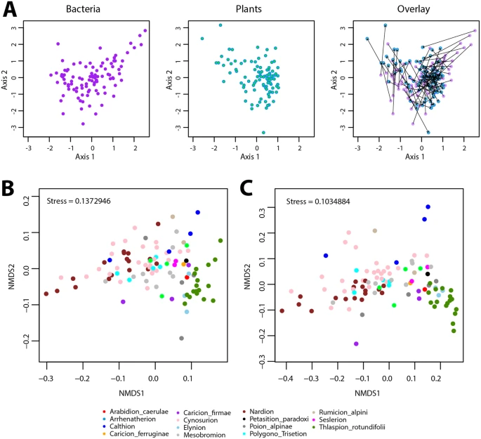 Figure1. Co-patterning of mountain grassland plant and bacterial communities. (A) Coinertia analysis based on the plant cover-abundance NMDS and bacterial community structure NMDS scores. The bacterial (purple) and plant (blue) components of the coinertia analysis are shown separately and overlaid across the ordination space for easier visualization, with arrows connecting bacteria and plant dots from the same site. (B) and (C) Co-patterning of bacterial communities per vegetation alliance, plotted in NMDS based on bacterial community structure and (C) on community membership. Dots (representing each site) are color-coded according to their prevailing vegetation alliance, but vegetation alliance information was not used for the NMDS calculation.
Plant communities were most strong driven by elevation, while soil bacteria were most strongly driven by soil pH (Figure 2). Bacterial diversity peaked at neutral pH, while plants diversity peaked at slightly acidic environments.
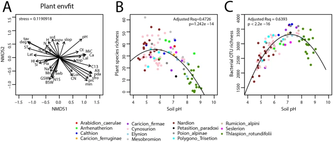 Figure2. Effect of abiotic factors on the plant and bacterial communities. (A) General effect of abiotic factors on the plant community structure, determined from the cover-abundance at each site and the environmental variables within the NMDS ordination space using envfit(). The arrows indicate the relative degree of and directionality of effect. The abbreviations of the soil physico-chemical and topo-climatic variables can be found in the original article. (B) Plant species richness and (C) bacterial OTU richness at each site plotted against soil pH. The dots are color-coded according to the vegetation alliance to which the sites belong.
The Nearest Taxon Index (NTI) values showed that sites with harsher environmental conditions had more overdispersed bacterial communities, and especially the Calthion vegetation habitat where the soil was anoxic and water-logged (Figure 3).
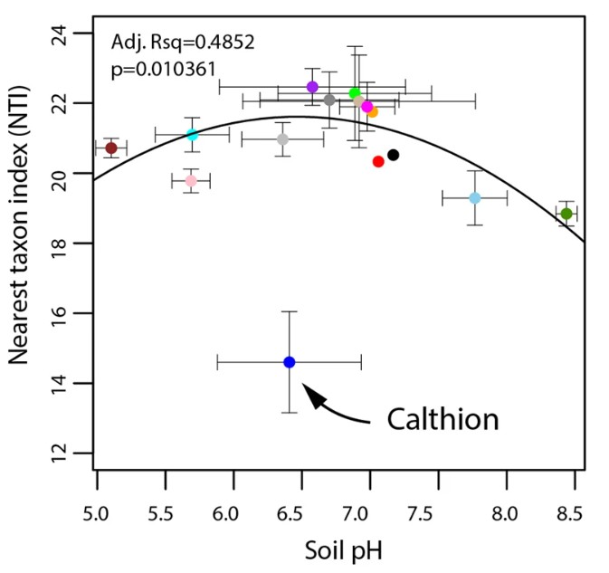 Figure 3. Effect of the environment on the evolutionary history of mountain grassland soil bacterial communities. The mean bacterial nearest taxon index (NTI) values across vegetation alliances is plotted against soil pH.
Generally, the more frequently occurring plant species were increased and decreased in abundance along with the more frequently occurring bacterial OTUs. These are considered as generalist species. The abundance of the less frequently occurring bacteria and plant species correlated with each other. Hence, we can observe clusters of specialist species in the co-occurrence network corresponding to the different plant habitats.
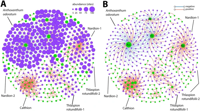 Figure 4. Correlation network analysis of the interactions among plant species and bacterial OTUs with node sizes in (A) indicating the number of sites where the plant species or bacterial OTU occurs, and (B) the degree of connectivity (i.e. number of edges). Plant species nodes are in green and bacterial OTU nodes in purple. Edges represent FDR-corrected positive (red) and negative (blue) Spearman correlations of ≥0.6 or ≤−0.6. Recognizable clusters are named according to the abundant plant names or vegetation alliance.
Figure 5 shows that the generalist plant and bacteria were strongly driven by soil pH (Figure 5 A and B). Removing the effect soil pH and elevation results in weaker plant-bacterial correlations, although the associations are still clearly present. The plant-bacterial associations in the water-logged anoxic Calthion sites were not affected by neither pH nor elevation.
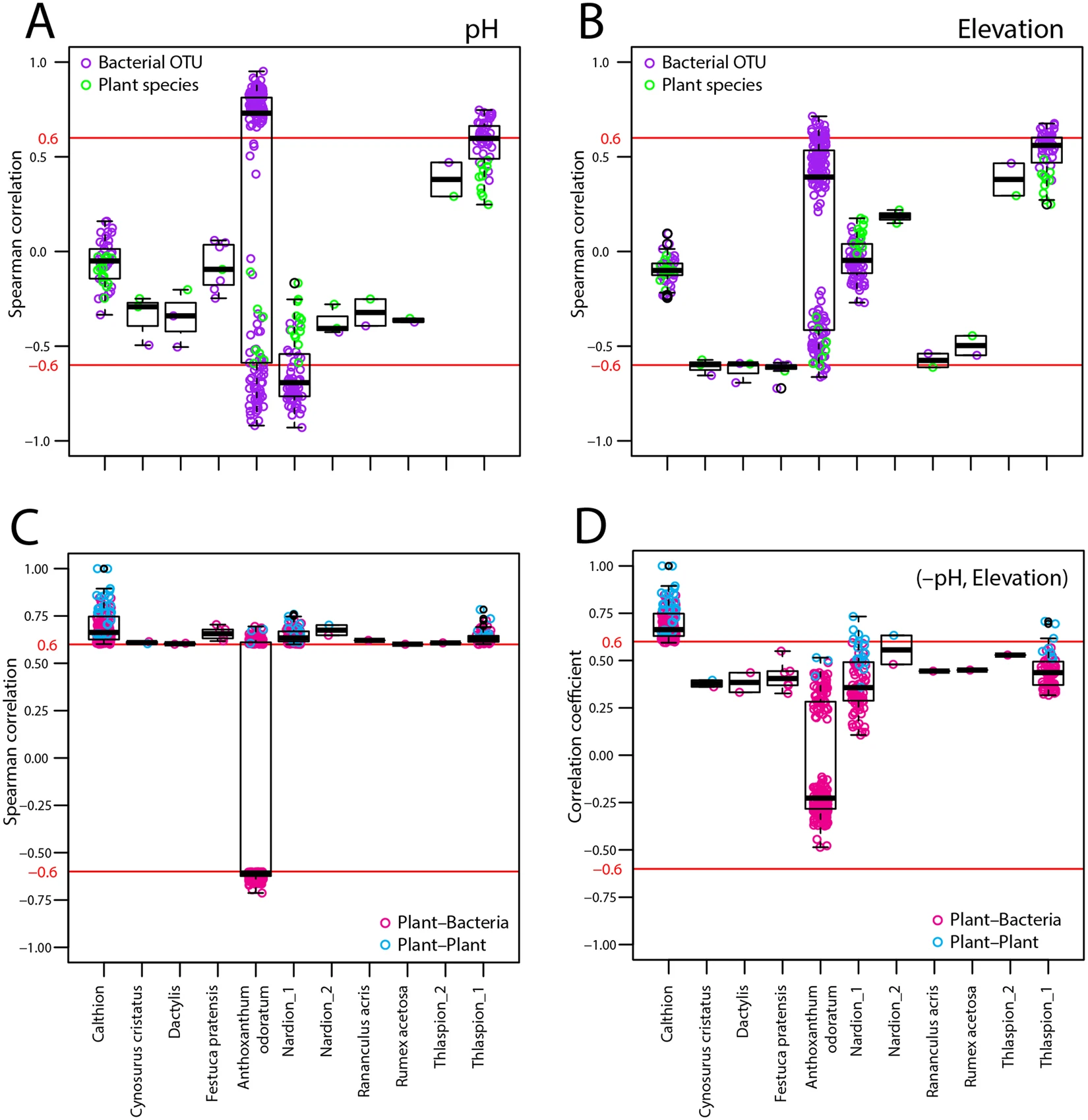 Figure 5. Dependence of bacterial OTU and plant species correlations within the respective correlation network clusters on underlying environmental variables. (A,B) Spearman correlations between plant species (green circles) and bacterial OTUs (purple) with soil pH or elevation. (C) Spearman correlations of plant-bacteria (magenta) and plant-plant (cyan) associations. (D) Partial Spearman correlations of (C) after removing the effect of soil pH and elevation. The red lines point to the thresholds, above or below which correlations are depicted in the earlier network.
~~~~~~~~~~~~~~~~~~
Differences in the diversity of mycobiomes associated with wheat processing and domestic environments
Yashiro, E., Savova-Bianchi D., Niculita-Hirzel, H. (2019) Major Differences in the Diversity of Mycobiomes Associated with Wheat Processing and Domestic Environments: Significant Findings from High-Throughput Sequencing of Fungal Barcode ITS1. International Journal of Environmental Research and Public Health 16(13): 2335 https://doi.org/10.3390/ijerph16132335
The fungal richness remained generally similar for the respective occupation groups during both periods of low and high exposure to dust.
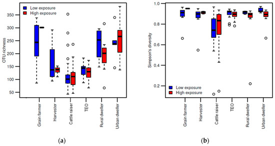
Figure 1. Fungal diversity among occupation groups according to the wheat dust exposure period: low or high. (a) Boxplot of OTU richness and (b) Simpson’s diversity among samples collected in the environment of each occupational group.
During periods when wheat workers were not exposed to wheat dust, the fungal community composition of the dust collected off of the workers was relatively similar to each other. During periods of high exposure to wheat dust, the fungal communitiy composition strongly different from profession to profession and among the different workplaces.
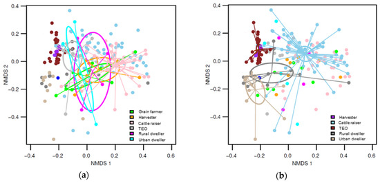
Figure 2. NMDS graphs of fungal communities with ordiellipses representing the 95% confidence intervals generated from the standard error. The communities from each occupation group are connected to the centroid by ordispider lines. (a) highlights the fungal communities from the period during low exposure to wheat dust, and (b) the communities from the high exposure period.
Grain farmers and urban and rural dwellers were associated with more group-specific OTUs than other wheat workers (Figure 3). The fewer group-specific indicator OTUs among the other wheat works also suggests that they harbor many of the same fungal OTUs.
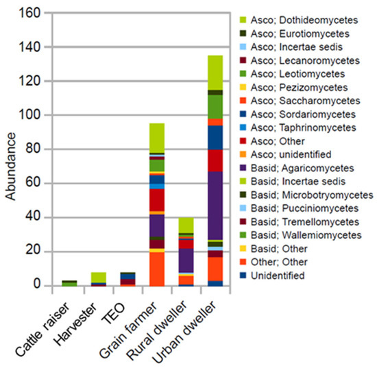
Figure 3 The mean relative abundance of each indicator OTU group at the fungal class level. The indicator OTUs were identified using Legendre and Legendre’s indicator species approach (R funcgion “indval”).
Professionals working with wheat were exposed to fungi known for their allergenic, toxigenic, or pathogenic effects. Not all of the pathogens were observer everywhere, and different known fungal pathogens were observed among workers in different professions.
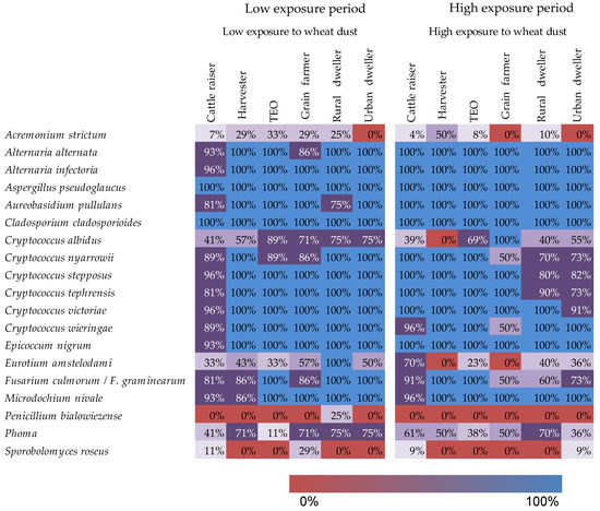
Figure 4. Heatmap illustrating the presence-absence of fungi of clinical importance as a functino of worker occupation and period of exposure to wheat dust. The colors and cell values indicate the proportion of samples in which the fungal species were detected.
~~~~~~~~~~~~~~~~~~
Fly population bottlenecks constrain the gut microbiome diversity and host genetic variation
Yashiro, E. and Ørsted, M., Hoffmann, A.A., Kristensen, T.N. (2022) Population bottlenecks constrain microbiome diversity and host genetic variation impeding fitness. PLOS Genetics 18(5): e1010206 https://doi.org/10.1371/journal.pgen.1010206
Note: Shared first authorship
The microbiome differred depending on the fly’s level of genetic variation. Also there was more ecological information contained in the bacterial community membership data (only ASV composition: unweighted UniFrac beta dissimilarity matrix) than in the community structure data (ASV composition + relative abundance: weighted UniFrac matrix). The lines across the ordination graphs show how the major host fly factors (viability and nuleotide diversity) correlate with the gut microbiome community composition.
Figure 1. Microbiome composition differ depending on the host’s level of genetic variation. NMDS plots based on the UniFrac distances. The 44 fly lines are color-coded as having low (red) and high (green) genetic variation and outbred (blue). The isolines are shown for host nucleotide diversity (A and C) and egg-to-adult viability (B and D). Envfit values (p < 0.05) are shown as arrows.
Certain bacterial ASVs and higher taxonomic groups are differentially abundant relative to the fly hosts’ level of genetic variation. The differential abundance of ASVs and higher taxonomic groups were identified using DESeq2 and plotted below.
Figure 2. Host genetic variation is associated with differential abundance of microbial taxa. Letters denote significant differences in relative abundance of ASVs and genera.
The core microbiomes of the low genetic variation fly lines are subsets of the high genetic variation lines.
Figure 3. Venn diagram showing the core microbiomes of the different groups of fly lines. The numbers denote the number ASVs that are shared or not shared among the fly lines.
Co-abundance network analysis shows that inbreeding is the likely the primary cause of a lower number of co-varying ASVs and decreased network complexity, regardless of the level of the hosts’ genetic variation.
Figure 4. Co-abundance networks of the fly microbiomes. The nodes are individual ASVs and the host fitness traits., while edges represent Spearman correlations. The network containing lines from all the fly groups (A and B), the outbred (C), high (D) and low (E) genetic variation groups are shown. The node sizes in A, C, D, and E